June 20, 2023
Share via

Part III: Data Science for Football

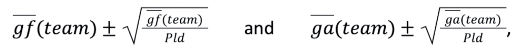
Most fans know that football teams often face strong performance fluctuations. One season, a Champions League qualification could seem possible, implying visits to some of Europe’s most legendary football arenas and millions of euros of extra earnings. The next season, there may be a serious risk of relegation, a financial shock which many clubs struggle to overcome. In such a season, the manager might be replaced several times. These fluctuations pose the question of whether it is really possible to judge performance from a few matches. Here, we discuss one of the simplest possible models to forecast the outcome of matches and a whole season. We base our modelling on two features only, the goals for (GF) and against (GA) each team during one season. These features are usually listed in football results tables.

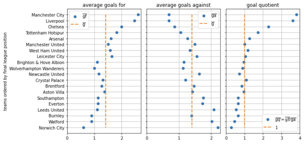
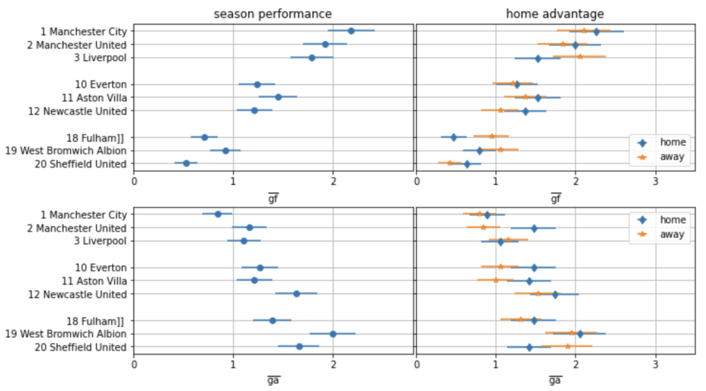
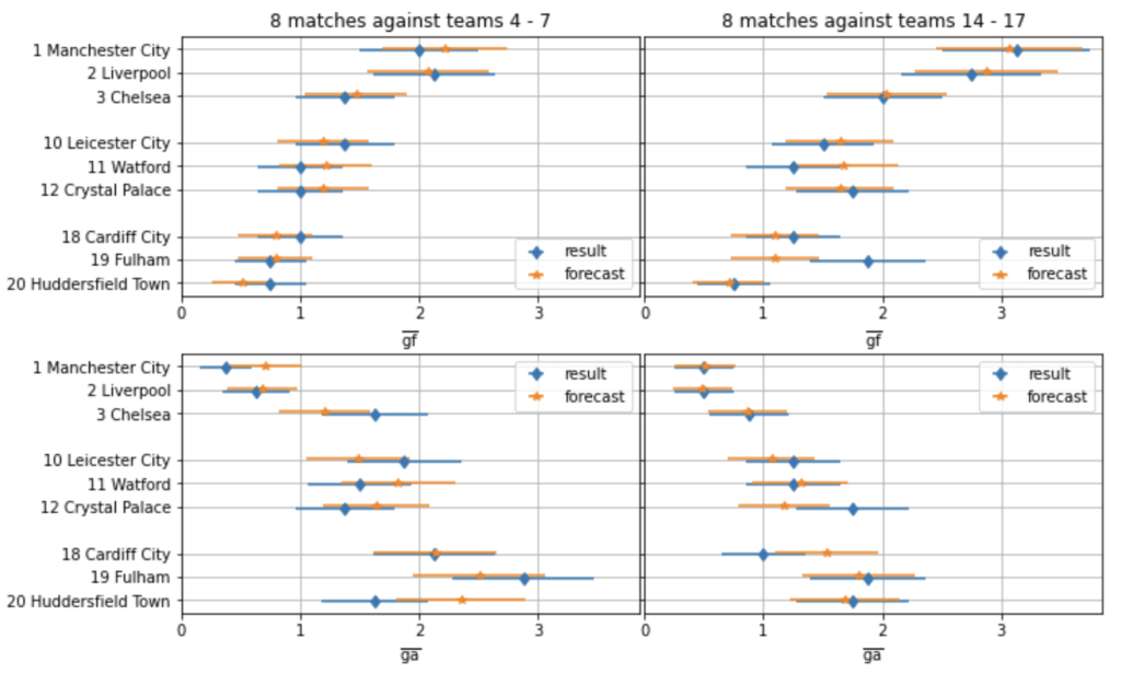
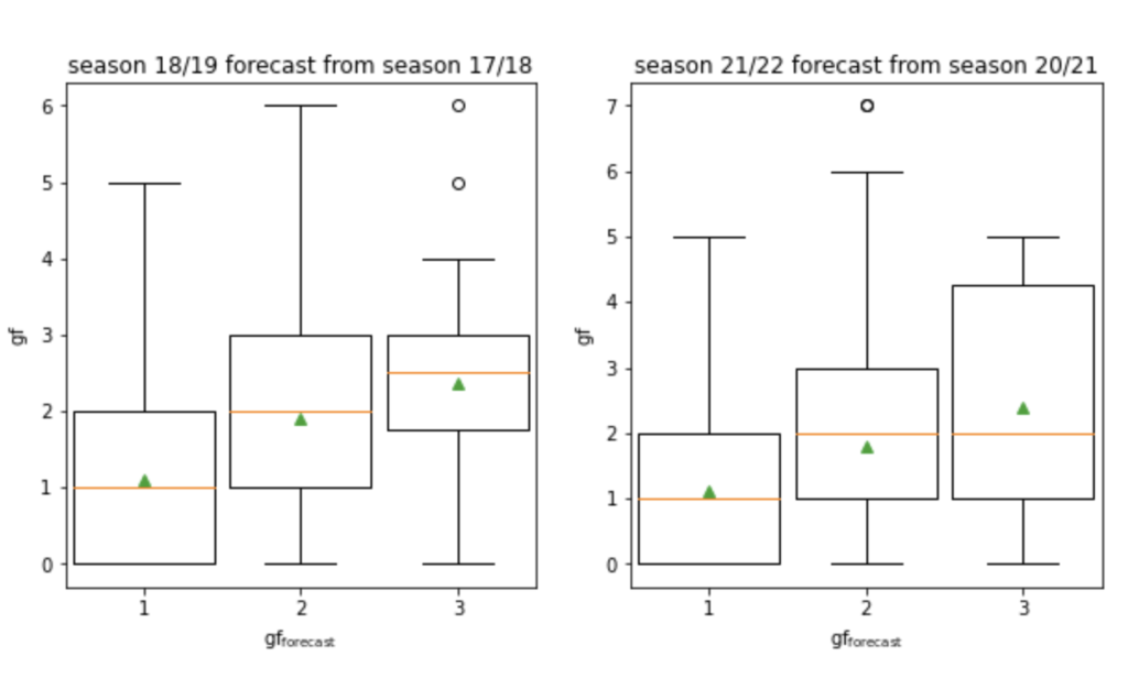
The exemplary table on the left of the following figure covers the 2021/22 Premier League season when twenty teams took part. The model will allow us to judge whether a team under- or over-performed over several matches by predicting the scoring probabilities for each team over all matches played.

 
The lower right of the figure lists two examples. Focusing on the Liverpool versus Arsenal matches —regardless of which team plays at home, Arsenal is expected to score zero goals with a large probability of 46%, while Liverpool is most likely to score two goals, with a probability of 27%. We will test forecast outcomes against match results of the same season (upper right of the figure, example match outcome Liverpool 4 – Arsenal 0). 
 
The model also allows us to forecast the next season (2022/23) with accuracy comparable to that of sports betting quotes. Based on past seasons we can show that such forecasts perform surprisingly well, so forecasts for the ongoing season should work effectively.


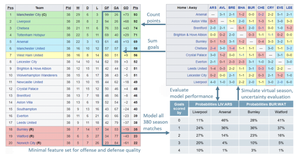
Data preparation and modeling logic

Before we start with our modelling efforts, let us first prepare the input data. The model should work for any league, regardless of the number of matches played. Therefore, we construct scalable metrics such as average goals for (gf) and against a team (ga) per match and a goal quotient, GQ, the ratio of goals scored to goals conceded by each team. These features are comparable across leagues and samples (i.e. over a few games or across multiple seasons): 

Small letters indicate data for a single match. Large letters are used for data aggregated over multiple matches. 

Averaging gf or ga over all teams we arrive at the same number g

The following figure highlights enormous differences in the goals for and against each team. Teams scoring many goals concede little, and vice versa.  

Therefore, the goal quotient presented on the right of the figure varies even more strongly than the goals for and against the teams separately. 

The quotient however has an intuitive meaning. For example, Manchester City scores almost four times as many goals as it concedes, while the opposite holds for Norwich City. Conversely, the meaning of the goal difference is less intuitive, as it needs context for a proper interpretation, like the number of games played and the typical total amount of goals during matches. 

Our main task in this article is to develop a model forecasting how many goals a team will score in a certain match. For example: if Manchester City played against an average league opponent like Aston Villa, the best forecast would be gf (Manchester City) = 2.6 goals, because this is the average number of goals scored by Manchester City per match. What do we expect if Manchester City played against a team with a weak defense like Norwich City, who are far below the league average? We could simply correct our forecast with the quotient ga (opponent)/g. This quotient is close to 1 for an average league opponent like Aston Villa, but it is 1.6 for a weak opponent like Norwich City, increasing the number of Manchester City forecasted goals to 4.1. The simple product model writes this in a compact formula.

Switching team and opponent in this formula, we find that Norwich City is expected to score about 0.3 goals against Manchester City on average. This is, at the same time, the forecasted number of goals against Manchester City, so the same model can be used to forecast the goals against a team. The left of the figure below illustrates the goal difference predicted by the model for every match in the league.

On the right of the figure we see how well the model performs. For every single match of the season, we compare gf forecast  and the number of goals gf which were actually scored in the match. The median is indicated with a horizontal orange line, the boxes mark the 25 (bottom) and 75-percentiles (top). 

Combining data from all the matches where about one goal was forecast, we see that the actual goals scored were most often zero, one or two. In a few cases, even up to five goals were scored. This says that it is very hard to forecast the number of goals exactly. Rather, the forecast tends to work on average. 

The average number of goals, indicated with a green triangle, is placed almost perfectly on the identity line gf forecast=gf across the plot range, which proves that the model works well on average. 

It is possible to model how likely it is, given gf forecast, that the actual number of goals gf is to take on the different values zero, one, two or more. This helps to estimate the uncertainty of the forecast. The details are not important for understanding further results presented here. It is enough to know the standard deviation connected to a certain forecast. Therefore, details about the goal distribution are presented in a box for readers interested in mathematics. 

Excurse for number crunchers: The goal distribution

We deal with the forecast uncertainty by modelling the number of goals with a Poisson distribution around gf forecast. The figure below displays data referring to the first and third bin plotted in the figure above. It indicates that the Poisson distribution works well for this purpose, because differences between Poisson and match data distribution are small. The Poisson distribution plays a major role in all kinds of count statistics like for example in describing radioactive decay statistics or particle collision events in physics. Therefore, it is well suited to counting goals. This distribution depends only on one parameter, being identical to the mean and variance of the distribution at the same time. Setting this parameter to  gf forecast, we find for the probability p of gf taking on a particular value: 

Let us calculate the uncertainty of the input features GF and GA. If we assume a constant offense and defense quality of each team over the season, match outcomes are still ruled by chance. Even a top team can sometimes score zero goals against one of the relegation candidates. For a single game we know from the properties of the Poisson distribution:  

mean(gf)=variance(gf)=gf forecast. Averaging the mean(gf) over all the matches of a team we find gf(team). The calculation involves replacing gf forecast individually for each match with the defining product formula. This result tells us that our model passes the self-consistency check. The variance of this average value is gf (team)/Pld, using the central limit theorem. Therefore the 68% confidence interval for the real intrinsic offense power of a team is

This confidence interval is valid in the Gaussian limit of large numbers, but the approximation works fine at around GF(team)= gf (team) Pld=10. 

Modelling results

The figure below covers the 2018/19 Premier League season. It was chosen because it was the last season not affected by COVID-19. The team’s final league position is given for three top teams, three mediocre teams and the three relegated teams.

We see how our goal forecast model enables us to calculate the uncertainty of goal counts:

The error bars indicate the intervals 

where the team’s estimated average goals per match are located. These ranges correspond to a 68% confidence interval. 

On the right of the figure, we see a clear home advantage for four of the nine teams in the offense (more goals scored home than away) and for two teams in the defense (less goals conceded home than away).

Goals for the top two teams have overlapping error bars meaning that there is no statistically significant difference in the offense quality of those two teams (left of the figure). The same holds for the goals against the teams, and indeed they collected almost the same points (Manchester City with 98 points, Liverpool with 97 points). Compared to them, Chelsea had a significantly weaker offense and defense, with error bars even overlapping those of mediocre teams, meaning that Chelsea was on a lower level. 

The mediocre teams are all on the same level, and their offense is significantly better than the offense of the relegated teams. The final league position of Chelsea was clearly only possible because of excellent home results, while away results were on the same level as mediocre teams. 

During the 2020/21 season, which was strongly affected by COVID-19, most of the matches were played without spectators. With the figure below we see that this modus undermined the home advantage. 

Teams usually building on a strong home advantage even had an “away advantage”, so Liverpool scored more goals away than at home, and Manchester United conceded less goals away than at home. 

If we want to evaluate the performance of a new manager during, for example, the first eight matches of their reign, it could be that the manager is unfortunate and only plays against top teams in that span. In this case it would be expected that the team scores less and concedes more than on average. The solution would be to compare results against the forecasted number of goals, as in the figure below for the season 2018/19. 

A scenario with matches against opponents from the better half of the league is presented on the left. Another scenario with opponents out of the weaker half is on the right. 

Error bars are much larger compared to previous figures, as we are now dealing with a smaller sample compared to a full, 38-game season. 

All teams are forecasted to score more and concede less goals against the weaker teams than against the stronger ones. The largest difference is that Manchester City is expected to score almost one more goal per match against the weaker teams (league positions 14 to 17) than against the stronger ones (league positions 4 to 7). In fact, Manchester City scored even more than one goal extra per match against the weaker teams. 

There is no team clearly over- or under-performing during this eight-match sample. The strongest over-performance is by the offense of Fulham against the weaker teams, scoring almost one extra goal per match compared to the forecast. This could indicate that Fulham was trying to fight relegation by taking the matches against other relegation candidates more seriously. Such a strategy doubles the impact, as it potentially increases Fulham’s points and decreases the points of opponents which could still fall behind Fulham. Anyhow, the result is not conclusive. Error bars slightly overlapping like that have an occurrence probability of more than 1/20, so for goals for and against the 9 displayed teams it is likely that we might observe such a case just by chance. Such a result could however still hint at a real underlying effect which could be evaluated with further statistical tests based on further features. 

As a final step let us see how the forecasts perform over subsequent seasons. The figure below provides forecasts for two different seasons from results of the previous season. In both cases, the three relegated teams were simply replaced by the new joiners who took possession of the goals for and goals against of those teams of the season before. The trend reproduces well. 

Deviations of binned results from the perfect identity reflect changes in the team’s quality over time. The better the forecast performs, the stronger the continuity of all teams from one season to the next. This fact could also be used to compare seasons with a larger time difference in between, to monitor changes in the league over time. 

Conclusion

Summarising, we constructed a simple model to forecast the number of goals during matches based on two features: the goals for and against the team during the whole season. This model allowed us to evaluate the uncertainty of results. This further enabled us to test whether there is a significant home advantage, and whether teams under- or over-perform in several matches, where the opponents can be a bad representation of the whole league by either being all top teams or all relegation candidates. The model also shows a good performance in forecasting the next season. 

There are many more insights to gather with this model, allowing us to add a small series of further articles:

  • Identifying significant over- or underperformance of teams with or without a certain player on the pitch, with a new manager or during the start of a season. 
  • The probability of winning, drawing or losing a match and the expected number of points collected per game are dependent in a simple way on the goal quotients of the teams involved. 
  • The probability for each team to be relegated or to qualify for the Champions League can be estimated from virtual runs of the season -> financial risk modelling. 
  • How a strengthened offense with an additional striker translates into additional points and increases the likelihood of qualifying for the Champions League can be quantified with the model. 
  • Using the forecasts for sports betting tasks and comparison with quotes from betting offices. 

Data Science & Football

This article is part of a three-part series that focuses on data science in relation to football.

To learn more about data science in football, you can also read these articles:

Part I: Deconstructing a Winning Season 

Part II: Evaluating Football Players

Details

Title: Bad Performance or Bad Luck? How Offense/Defense Quality and Uncertainty Impact Outcomes in Football
Author:
DAIN Studios, Data & AI Strategy Consultancy
Published in ,
Topics:
Updated on January 27, 2024