Computer Vision API: Setting up the environment
The requirements for creating a Computer Vision API are straightforward. You need a Google account in order to able to access your Google Drive and use Google Colab.
1. Create your Image Dataset
We are going to classify flowers but, instead of taking existing datasets available from the Internet, we are going to build our own labeled image dataset using Google Images.
First, open your new notebook Google Colab and connect it to your drive with the following code:
from google.colab import drive
drive.flush_and_unmount()
drive.mount('/content/gdrive', force_remount=True)
root_dir = "/content/gdrive/My Drive/"
You will be asked to click a link and copy/past the code that will be given to you in the box appearing in the output of the cell.
Now you can access the data in your Drive from your notebook.
Download the images and store them into your Drive. To do this, go on Google Image and search for the objects you want to classify. In our case, we want to classify Sunflower, yellow Daisy and yellow Tulip. Let’s start with the Sunflowers. Search Sunflowers on Google image and scroll to the bottom until you see show more results. Then, open the developer mode of your browser and go the Web Console.
There, paste the following code to download a CSV of all the image urls:
urls = Array.from(document.querySelectorAll('.rg_di .rg_meta')).map(el=>JSON.parse(el.textContent).ou);window.open('data:text/csv;charset=utf-8,' + escape(urls.join('\n')));This triggers the download of the file. Save it and upload it using the widget on the left of the Notebook: Files > Upload. Do the same for the other flowers.
We are going to now use the fast.ai library. Create a cell and paste:
!curl -s https://course.fast.ai/setup/colab | bashThis will install the library and configure your Colab notebook to run smoothly with it. Then, activate the GPU going to Runtime > Change Runtime Type > GPU.
2. Download data
Now, import the library and download the images:
from fastai.vision import *
from fastai.metrics import error_rate
In [0]:
folders_files = [('sunflowers', 'sunflowers.csv'), ('yellow_daisy', 'yellow_daisy.csv'), ('yellow_tulips', 'yellow_tulips.csv')]
for (folder, file) in folders_files:
  path = Path('/content/gdrive/My Drive/DeepLearning/Datasets/')
  folder = (path/folder)
  folder.mkdir(parents=True, exist_ok=True)
  download_images(path/file, folder, max_pics=200)
  verify_images(folder, delete=True, max_size=500)
Here we create a folder and download 200 images for each class and verify they are not corrupted.
Next, we create an ImageDataBunch from the downloaded images. This object will represent our data with their labels. To optimise the process, we also:
- Split the data to have 20% of validation
- Resize the data in squares of 224 pics
- Operate image augmentation with get_transforms
- Normalize the data
np.random.seed(42)
data = ImageDataBunch.from_folder(path, train=".", valid_pct=0.2,
        ds_tfms=get_transforms(), size=224, num_workers=4).normalize(imagenet_stats)
3. View data
Let’s visualize our data:
data.show_batch(rows=3, figsize=(7,6))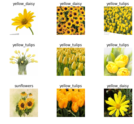
Everything seems correct. However to ensure optimal performance, you should check the images manually and remove the non-consistent images from your dataset. The Google Drive UI is quite convenient for validating and filtering images manually.
4. Train model
Now we are going to train our model. The fast.ai library is concise and is set with good default features.
learn = cnn_learner(data, models.resnet34, metrics=error_rate)
learn.fit_one_cycle(4)
Downloading: “https://download.pytorch.org/models/resnet34-333f7ec4.pth” to /root/.cache/torch/checkpoints/resnet34-333f7ec4.pth 100%|██████████| 87306240/87306240 [00:00<00:00, 109355856.48it/s]
| epoch | train_loss | valid_loss | error_rate | time |
| 0 | 0.890968 | 0.387459 | 0.138528 | 0:28 |
| 1 | 0.527052 | 0.283305 | 0.064935 | 0:18 |
| 2 | 0.378353 | 0.281448 | 0.064935 | 0:18 |
| 3 | 0.282371 | 0.271847 | 0.060606 | 0:18 |
With these lines, we are downloading a pre-trained model ResNet34, passing our data and setting the metric as the error rate.
Then, we fit the model with the one cycle policy, as this mode of approach usually performs well.
We get an error rate of 6% which is not bad, but we could do better. We were training the top layers of the pre-trained model. Let’s unfreeze all layers so their parameters are able to be modified during the training phase.
learn.unfreeze()fast.ai library provides lr_find which will launch an LR range test that will help you select a good learning rate. Plotting the curve:
learn.lr_find()
learn.recorder.plot()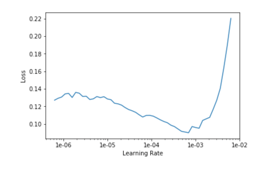
A rule thumb is to spot the strongest downward slope. Therefore we pick the beginning of the range at 1e-5 and choose to stop at 1e-4 because we were already training at 1e-3 by default. That way, the first layers are will be trained with a learning rate of 3e-5 and the last ones at 3e-4.
learn.fit_one_cycle(10, max_lr=slice(3e-5,3e-4))| epoch | train_loss | valid_loss | error_rate | time |
| 0 | 0.13375 | 0.250481 | 0.056277 | 0:18 |
| 1 | 0.094298 | 0.215684 | 0.038961 | 0:19 |
| 2 | 0.068966 | 0.253927 | 0.038961 | 0:19 |
| 3 | 0.052962 | 0.270199 | 0.034632 | 0:18 |
| 4 | 0.039442 | 0.25092 | 0.034632 | 0:19 |
| 5 | 0.032108 | 0.251597 | 0.034632 | 0:18 |
| 6 | 0.028615 | 0.254128 | 0.034632 | 0:19 |
| 7 | 0.022683 | 0.250784 | 0.034632 | 0:19 |
| 8 | 0.018629 | 0.257523 | 0.034632 | 0:18 |
| 9 | 0.015092 | 0.253845 | 0.034632 | 0:18 |
3.5% error, which is better.
Let’s analyze the classification errors:
interp = ClassificationInterpretation.from_learner(learn)
interp.plot_confusion_matrix(figsize=(12,12), dpi=60)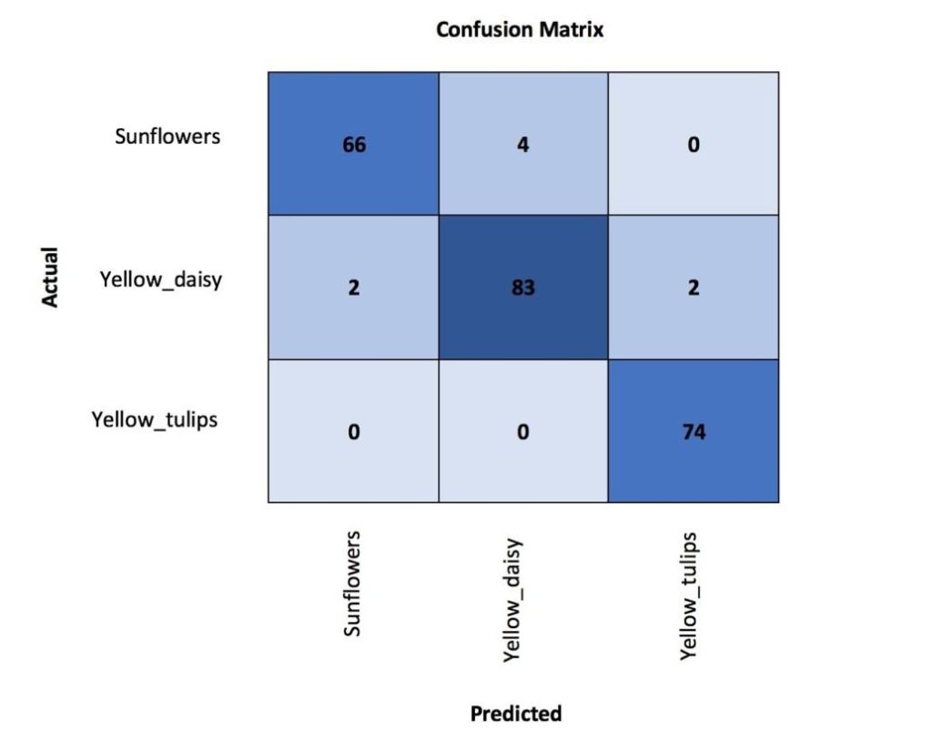
We see most of the errors come from the confusion between yellow daisy and sunflowers which can be understandable due to their visual similarities. Plotting the errors which had the biggest top loss can help us to further understand the causes of the error.
interp.plot_top_losses(9, figsize=(15,11))
Some normal images have been misclassified, but others don’t look like flowers at all. This process demonstrates that we have not cleaned the dataset to the extent that we should have. Therefore, to improve performance, we should clean the image dataset and rerun the process to have a consistent score.
After cleaning and retraining our model, it should be a shame to keep it in the notebook, let’s put it in production!
5. Export the API model to production
Save your model:
learn.export()Download it and save it at the base of your API local folder. We are going now to build a basic API which will allow the user to upload an image and get the prediction.
Create a virtual environment with Python 3 having Flask and fast.ai library.
Create api_endpoint.py and past the following code:
import os
from flask import Flask, flash, request, redirect, url_for, send_from_directory, jsonify
from werkzeug.utils import secure_filename
from fastai.vision import *


app = Flask(__name__)

UPLOAD_FOLDER = os.getcwd() + '/files/'
ALLOWED_EXTENSIONS = {'png', 'jpg', 'jpeg', 'gif'}

app = Flask(__name__)
app.config['UPLOAD_FOLDER'] = UPLOAD_FOLDER


def allowed_file(filename):
    return '.' in filename and \
           filename.rsplit('.', 1)[1].lower() in ALLOWED_EXTENSIONS

@app.route('/', methods=['GET', 'POST'])
def upload_file():
    if request.method == 'POST':
        # check if the post request has the file part
        if 'file' not in request.files:
            flash('No file part')
            return redirect(request.url)
        file = request.files['file']
        # if user does not select file, browser also
        # submit an empty part without filename
        if file.filename == '':
            flash('No selected file')
            return redirect(request.url)
        if file and allowed_file(file.filename):
            filename = secure_filename(file.filename)
            img = open_image(file)
            pred, _, losses = learner.predict(img)
            print(pred)
            file.save(os.path.join(app.config['UPLOAD_FOLDER'], filename))
            return jsonify(str(pred))
    return '''
    <!doctype html>
    <title>Upload new File</title>
    <h1>Upload new File</h1>
    <form method=post enctype=multipart/form-data>
      <input type=file name=file>
      <input type=submit value=Upload>
    </form>
    '''

@app.route('/uploads/<filename>')
def uploaded_file(filename):
    # return send_from_directory(app.config['UPLOAD_FOLDER'],
    #                            filename)
    return 'File updated!'

if __name__ == '__main__':
    defaults.device = torch.device('cpu')
    learner = load_learner('.')
    print('OK')
    app.run(host="0.0.0.0", port=int("80"), debug=True)
Launch your API with python api_endpoint.py and access with http://0.0.0.0/
There you can upload your image and get your classification. For example with this image:
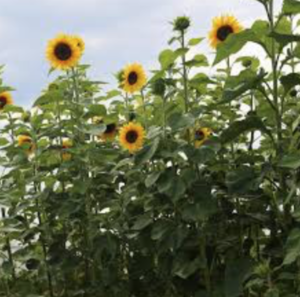
As a return result we have the following JSON:
{
"sunflower"
}
6. Next steps
To go deeper into computer vision and API building, I highly recommend you try the excellent courses of https://www.fast.ai/.
You can check the code in the DAIN Studios’ GitHub repository
Written by Thomas Nguyen, a Data Engineer at DAIN Studios based in Berlin, Germany.